Do Rectifier Efficiency Differences Matter in Continuous Operation?

Are rectifier efficiency differences significant in continuous operation? Yes—especially when equipment supplies substantial DC power around the clock. A small efficiency gap can become a meaningful electricity expense and a persistent heat load. But the difference between two headline ratings is not enough to decide which unit deserves the budget.

A rectifier operating near its best-efficiency point all year presents a different purchasing problem from an oversized redundant system spending most of its life lightly loaded. Output voltage, ambient temperature, cooling arrangements, and the measurement boundary can all change the result. The useful question is not simply which rectifier is more efficient, but how much less energy it will consume while delivering the same service.

Start with losses, not the percentage-point gap

Rectifier efficiency is DC output power divided by AC input real power. For a fixed DC load, the lower-efficiency unit draws more input power, and most of that difference becomes heat within the equipment. Calculate losses using:

Power loss = DC output power × (1 ÷ efficiency − 1)

Use efficiency as a decimal. Also check what the specification includes: a semiconductor bridge efficiency figure is not interchangeable with the AC-to-DC efficiency of a complete cabinet containing transformers, filters, controls, and fans.

Consider an illustrative comparison—not a claim about any particular product. Two complete rectifiers continuously deliver 100 kW of DC output. One operates at 96% efficiency and the other at 97%, under identical conditions.

• The 96% unit draws approximately 104.17 kW and loses 4.17 kW.
• The 97% unit draws approximately 103.09 kW and loses 3.09 kW.
• The input-power difference is approximately 1.07 kW.
• Across 8,760 operating hours, that difference represents approximately 9,407 kWh.

At an assumed electricity price of $0.12/kWh, the annual energy saving is approximately $1,129, excluding cooling and other tariff effects. The efficiency improvement is only one percentage point, yet rectifier losses fall by roughly 26%. That distinction matters when evaluating cabinet ventilation or electrical-room heat removal.

Do not calculate the saving as 1% of annual DC energy. At a fixed output, the correct comparison uses the reciprocal efficiencies, as above.

Replace the nameplate assumption with a load profile

Continuous operation does not mean constant load. A telecom DC plant may remain energized continuously while its demand changes. A charging installation may experience high charging current after a discharge, followed by extended float operation. An industrial process rectifier may run throughout a shift but change current or voltage with production requirements.

Each case needs a different efficiency comparison. Fixed consumption from controls and auxiliary circuits becomes more influential at low output. Conduction losses increase with current, while switching and magnetic losses depend on the design and operating point. A unit with the better peak rating can therefore lose its advantage elsewhere on the curve.

Build a simple operating-hours distribution from logged data. Group the year into representative combinations of output power, output voltage, and temperature. For each group, calculate:

Energy saving = output power × operating hours × (1 ÷ efficiency A − 1 ÷ efficiency B)

Add the groups together. This is more reliable than inserting an arithmetic average efficiency into the annual calculation. For variable-voltage process supplies, power alone may not adequately describe the operating point: obtain efficiency data at the actual voltage and current combinations.

Redundancy deserves particular attention. In an N+1 modular system, sharing a modest load across every installed module can put each module at an inefficient operating point. Module-sleep controls may improve performance, but their reserve capacity, wake-up response, and behavior during faults must satisfy the application. Energy optimization should not quietly reduce the resilience the system was purchased to provide.

Check where the heat goes

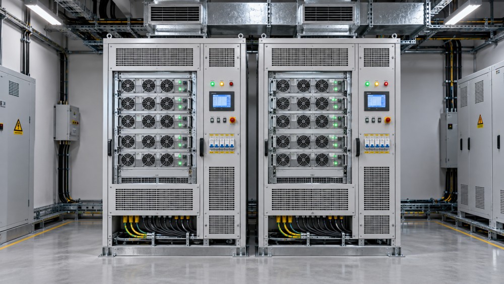
In the 100 kW example, the more efficient rectifier releases approximately 1.07 kW less heat. Whether that creates additional electricity savings depends on the installation. In an air-conditioned electrical room, mechanical cooling may consume less power. In a naturally ventilated enclosure, there may be little direct cooling-energy saving, although the reduced thermal burden can still be useful.

Where mechanical cooling serves the room, estimate the incremental cooling electricity from the avoided heat and the cooling system’s actual operating performance. Do not apply a generic multiplier without checking seasonal conditions, control behavior, and whether the cooling plant can reduce its consumption at that load.

Lower losses can also help preserve thermal margin around capacitors, magnetic components, and power semiconductors. That is not proof of longer service life. A compact high-efficiency design can still have demanding internal temperatures, and fan failure or restricted airflow can overwhelm an otherwise attractive efficiency figure.

For hot or dusty locations, review the derating curve, permitted inlet temperature, filter maintenance, and airflow requirements alongside efficiency. A rectifier that meets its rating only with unusually cool inlet air may be the wrong choice for an existing equipment room.

Make supplier comparisons genuinely equivalent

A quoted “up to” efficiency is a useful starting point, not a purchasing conclusion. Before comparing bids, request supporting data that resolves these questions:

• What is included? Confirm whether fans, controls, input magnetics, filters, and external auxiliaries fall inside the measurement boundary.
• At which electrical conditions? Match AC input voltage and frequency, DC output voltage, load, and any relevant ripple requirements.
• Under which thermal conditions? Establish ambient or inlet temperature, warm-up time, and whether cooling equipment was operating normally.
• How does the complete system behave? Obtain data for the proposed module population and redundancy strategy, not just one module at its optimum point.
• How certain is the result? Ask for the test method, instrument accuracy, and measurement uncertainty where differences are small.

Power factor is a separate issue. It describes the relationship between real and apparent input power; it is not conversion efficiency. High power factor can help with upstream capacity and certain tariff arrangements, but it does not establish that the rectifier has low internal losses. Harmonic current, electromagnetic compatibility, output ripple, and transient performance likewise need their own acceptance criteria.

Technology labels are not substitutes for these measurements. Active front ends, synchronous rectification, and wide-bandgap devices can enable useful improvements, but their benefit depends on the complete design. More sophisticated conversion also brings control, protection, serviceability, and cost considerations.

Put a defensible limit on the efficiency premium

Simple payback provides a quick screening calculation: divide the additional installed cost by the annual net saving. Include installation differences, not just the equipment-price difference. A premium of $4,000 against the illustrative $1,129 annual electricity saving would have a simple payback of about 3.5 years before cooling, maintenance, financing, or discounting.

For a longer-life asset, compare discounted lifecycle costs using the organization’s investment assumptions. Test a lower-load case as well as the expected operating profile. If the proposal works only with uninterrupted full-load operation and rising electricity prices, the business case is fragile.

Demand-charge savings require separate analysis. A reduction in rectifier input power lowers the billable peak only if it affects the tariff’s relevant measurement period and conditions. Similarly, emissions savings should use a documented electricity emissions factor appropriate to the reporting purpose, rather than an unsupported universal conversion.

For an existing installation, replacement is a harder decision than selecting between new units. Remaining service life, shutdown risk, spares, commissioning, and the condition of the current equipment can outweigh modest energy savings. For a new continuously loaded plant, the same efficiency premium may be straightforward to justify.

Verify the operating point before committing

For a consequential purchase, agree on a witnessed test or an acceptance procedure at representative loads. Measure AC real input power and DC output power simultaneously after thermal stabilization. Use instruments suited to the waveforms involved; multiplying nominal voltage by displayed current is not an adequate efficiency test. Significant ripple may also require waveform-aware output-power measurement.

Avoid claiming precision that the measurement setup cannot support. Subtracting two large readings to establish a small loss difference makes instrument uncertainty especially important. Record auxiliary consumption and test conditions so that later site readings remain comparable.

This equipment-to-system perspective fits the Global Power & Electrical Grid Matrix’s focus on connecting power-electronics developments with practical grid and industrial investment decisions. The valuable intelligence is not simply that conversion technology is improving; it is knowing which improvement survives the project’s load profile, thermal conditions, and commercial constraints.

For continuously operated rectifiers, efficiency differences often do matter. Before paying for the better number, obtain the efficiency curve at your operating voltage, establish annual hours at each load, and price the resulting loss difference. If those inputs are missing, the next step is to request them—not to assume the peak rating represents the coming decade of operation.